import pandas as pd
import numpy as np
import matplotlib.pyplot as plt
import seaborn as sns
from sklearn.linear_model import LogisticRegression
from sklearn.model_selection import train_test_split
from sklearn.metrics import classification_report, confusion_matrix
from sklearn.preprocessing import StandardScaler
import statsmodels.api as sm

np.random.seed(123)

email = pd.read_csv('data/email.csv')AE 11: Building a spam filter
In this application exercise, we will
- Use logistic regression to fit a model for a binary response variable
- Fit a logistic regression model in Python
- Use a logistic regression model for classification
To illustrate logistic regression, we will build a spam filter from email data.
The data come from incoming emails in David Diez’s (one of the authors of OpenIntro textbooks) Gmail account for the first three months of 2012. All personally identifiable information has been removed.
print(email.info())
print(email.describe())
<class 'pandas.core.frame.DataFrame'>
RangeIndex: 3921 entries, 0 to 3920
Data columns (total 21 columns):
# Column Non-Null Count Dtype
--- ------ -------------- -----
0 spam 3921 non-null int64
1 to_multiple 3921 non-null int64
2 from 3921 non-null int64
3 cc 3921 non-null int64
4 sent_email 3921 non-null int64
5 time 3921 non-null object
6 image 3921 non-null int64
7 attach 3921 non-null int64
8 dollar 3921 non-null int64
9 winner 3921 non-null object
10 inherit 3921 non-null int64
11 viagra 3921 non-null int64
12 password 3921 non-null int64
13 num_char 3921 non-null float64
14 line_breaks 3921 non-null int64
15 format 3921 non-null int64
16 re_subj 3921 non-null int64
17 exclaim_subj 3921 non-null int64
18 urgent_subj 3921 non-null int64
19 exclaim_mess 3921 non-null int64
20 number 3921 non-null object
dtypes: float64(1), int64(17), object(3)
memory usage: 643.4+ KB
None
spam to_multiple from cc sent_email \
count 3921.000000 3921.000000 3921.000000 3921.000000 3921.000000
mean 0.093599 0.158123 0.999235 0.404489 0.277990
std 0.291307 0.364903 0.027654 2.666424 0.448066
min 0.000000 0.000000 0.000000 0.000000 0.000000
25% 0.000000 0.000000 1.000000 0.000000 0.000000
50% 0.000000 0.000000 1.000000 0.000000 0.000000
75% 0.000000 0.000000 1.000000 0.000000 1.000000
max 1.000000 1.000000 1.000000 68.000000 1.000000
image attach dollar inherit viagra \
count 3921.000000 3921.000000 3921.000000 3921.000000 3921.000000
mean 0.048457 0.132874 1.467228 0.038001 0.002040
std 0.450848 0.718518 5.022298 0.267899 0.127759
min 0.000000 0.000000 0.000000 0.000000 0.000000
25% 0.000000 0.000000 0.000000 0.000000 0.000000
50% 0.000000 0.000000 0.000000 0.000000 0.000000
75% 0.000000 0.000000 0.000000 0.000000 0.000000
max 20.000000 21.000000 64.000000 9.000000 8.000000
password num_char line_breaks format re_subj \
count 3921.000000 3921.000000 3921.000000 3921.000000 3921.000000
mean 0.108136 10.706586 230.658505 0.695231 0.261413
std 0.959931 14.645786 319.304959 0.460368 0.439460
min 0.000000 0.001000 1.000000 0.000000 0.000000
25% 0.000000 1.459000 34.000000 0.000000 0.000000
50% 0.000000 5.856000 119.000000 1.000000 0.000000
75% 0.000000 14.084000 298.000000 1.000000 1.000000
max 28.000000 190.087000 4022.000000 1.000000 1.000000
exclaim_subj urgent_subj exclaim_mess
count 3921.000000 3921.000000 3921.000000
mean 0.080337 0.001785 6.584290
std 0.271848 0.042220 51.479871
min 0.000000 0.000000 0.000000
25% 0.000000 0.000000 0.000000
50% 0.000000 0.000000 1.000000
75% 0.000000 0.000000 4.000000
max 1.000000 1.000000 1236.000000 The variables we’ll use in this analysis are
spam: 1 if the email is spam, 0 otherwiseexclaim_mess: The number of exclamation points in the email message
Goal: Use the number of exclamation points in an email to predict whether or not it is spam.
Exploratory data analysis
Let’s start by taking a look at our data. Create an density plot to investigate the relationship between spam and exclaim_mess. Additionally, calculate the mean number of exclamation points for both spam and non-spam emails.
# add code hereLinear model – a false start
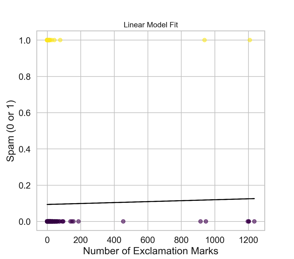
Suppose we try using a linear model to describe the relationship between the number of exclamation points and whether an email is spam. Write up a linear model that models spam by exclamation marks.
# add code hereA visualization of a linear model is below.
plt.figure(figsize=(8, 6))
plt.scatter(email['exclaim_mess'], email['spam'], alpha=0.5, c=email['spam'], cmap='viridis')
plt.plot(email['exclaim_mess'], linear_model.predict(sm.add_constant(X)), color='black')
plt.xlabel('Number of Exclamation Marks')
plt.ylabel('Spam (0 or 1)')
plt.title('Linear Model Fit')
plt.show()
- Is the linear model a good fit for the data? Why or why not?
Add response here.
Logistic regression – a different approach
Let \(p\) be the probability an email is spam (success).
- \(\frac{p}{1-p}\): odds an email is spam (if p = 0.7, then the odds are 0.7/(1 - 0.7) = 2.33)
- \(\log\Big(\frac{p}{1-p}\Big)\): “log-odds”, i.e., the natural log, an email is spam
The logistic regression model using the number of exclamation points as an explanatory variable is as follows:
\[\log\Big(\frac{p}{1-p}\Big) = \beta_0 + \beta_1 \times exclaim\_mess\]
The probability an email is spam can be calculated as:
\[p = \frac{\exp\{\beta_0 + \beta_1 \times exclaim\_mess\}}{1 + \exp\{\beta_0 + \beta_1 \times exclaim\_mess\}}\]
Exercises
Exercise 1
- Fit the logistic regression model using the number of exclamation points to predict the probability an email is spam.
X = email[['exclaim_mess']]
y = email['spam']

log_reg = LogisticRegression()
log_reg.fit(X, y)

# Summary output
print(f"Intercept: {log_reg.intercept_[0]}")
print(f"Coefficient: {log_reg.coef_[0][0]}")
Intercept: -2.2723427075496763
Coefficient: 0.0002724094404145483- How does the code above differ from previous code we’ve used to fit regression models? Compare your summary output to the estimated model below.
\[\log\Big(\frac{p}{1-p}\Big) = -2.27 - 0.000272 \times exclaim\_mess\]
Add response here.
Exercise 2
What is the probability the email is spam if it contains 10 exclamation points? Answer the question using the log_reg.predict_proba() function.
email_10_exclaim = np.array([[10]])
pred_prob = log_reg.predict_proba(email_10_exclaim)[0][1]
print(f"Predicted probability of spam for an email with 10 exclamation points: {pred_prob}")
Predicted probability of spam for an email with 10 exclamation points: 0.09367058559410353Exercise 3
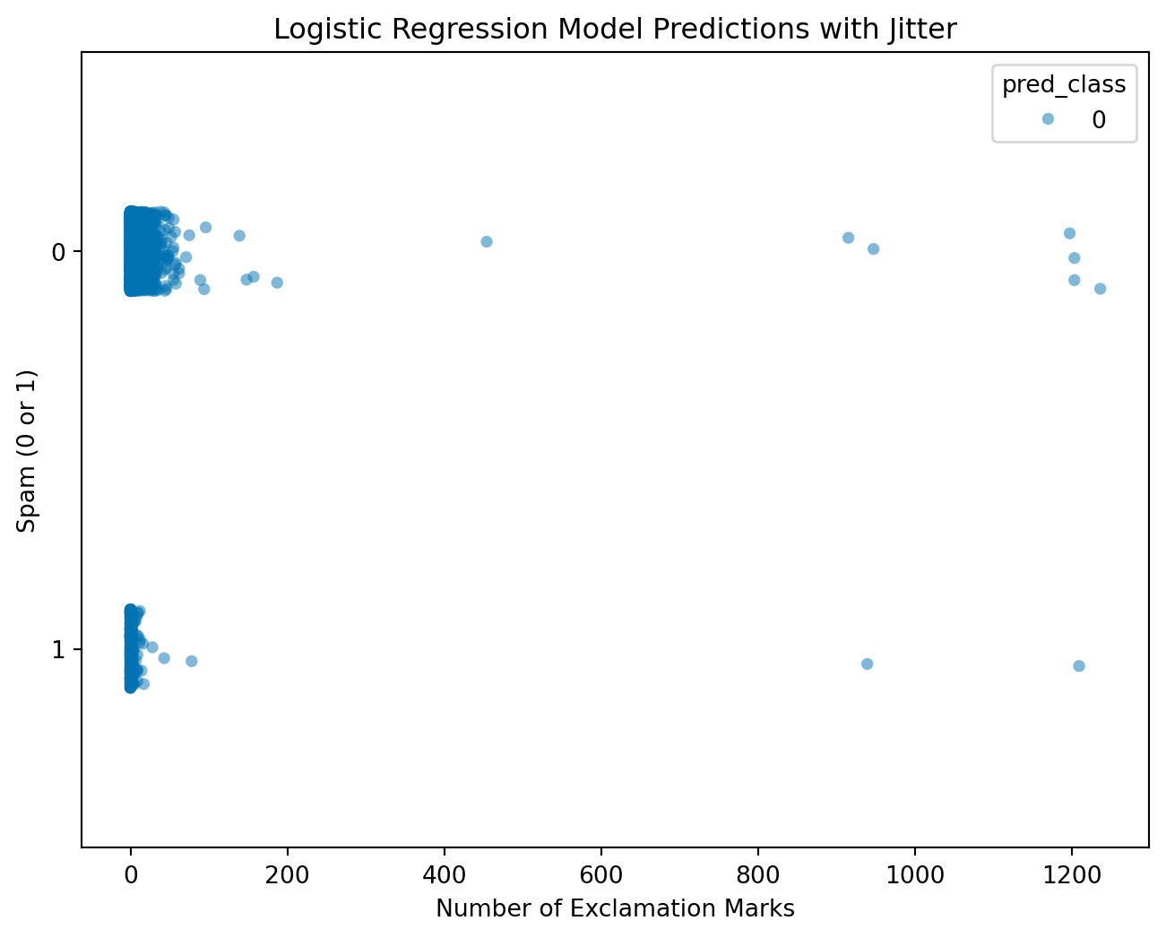
We have the probability an email is spam, but ultimately we want to use the probability to classify an email as spam or not spam. Therefore, we need to set a decision-making threshold, such that an email is classified as spam if the predicted probability is greater than the threshold and not spam otherwise.
Suppose you are a data scientist working on a spam filter. You must determine how high the predicted probability must be before you think it would be reasonable to call it spam and put it in the junk folder (which the user is unlikely to check).
What are some trade offs you would consider as you set the decision-making threshold?
Add response here.
email['pred_class'] = (log_reg.predict_proba(X)[:, 1] >= 0.5).astype(int)

plt.figure(figsize=(8, 6))
sns.stripplot(data=email, x='exclaim_mess', y=email['spam'].astype(str), hue='pred_class', palette='colorblind', jitter=True, alpha=0.5)
plt.xlabel('Number of Exclamation Marks')
plt.ylabel('Spam (0 or 1)')
plt.title('Logistic Regression Model Predictions with Jitter')
plt.show()
Exercise 4
Fit a model with all variables in the dataset as predictors and recreate the visualization above for this model.
# add code here- Use model evaluation metrics from
confusion_matrixandclassification_reportto evaluate our model.
# add code here