AE 11: Modelling loan interest rates

In this application exercise we will be studying loan interest rates. The dataset is one you’ve come across before in your reading – the dataset about loans from the peer-to-peer lender, Lending Club, from the openintro R package. We will use pandas and scikit-learn for data exploration and modeling, respectively.

import pandas as pd
import numpy as np
import matplotlib.pyplot as plt
import seaborn as sns
from sklearn.linear_model import LinearRegression
from sklearn.metrics import mean_squared_error
import statsmodels.api as sm
import statsmodels.formula.api as smf

loans = pd.read_csv('data/loans_full_schema.csv')

Before we use the dataset, we’ll make a few transformations to it.

• Your turn: Review the code below and write a summary of the data transformation pipeline.

Answer:
The code performs several data cleaning and feature engineering steps: - Creates credit_util as a ratio of credit used to total credit limit. - Transforms public_record_bankrupt into a binary categorical variable bankruptcy. - Converts verified_income and homeownership to categorical variables, with homeownership set as an ordered category. - Renames inquiries_last_12m to credit_checks. - Filters the dataset to retain only the relevant variables for analysis.

loans['credit_util'] = loans['total_credit_utilized'] / loans['total_credit_limit']
loans['bankruptcy'] = loans['public_record_bankrupt'].apply(lambda x: 0 if x == 0 else 1).astype('category')
loans['verified_income'] = loans['verified_income'].astype('category')
loans['homeownership'] = loans['homeownership'].str.title().astype('category')
loans['homeownership'] = pd.Categorical(loans['homeownership'], categories=["Rent", "Mortgage", "Own"], ordered=True)
loans = loans.rename(columns={'inquiries_last_12m': 'credit_checks'})
loans = loans[['interest_rate', 'loan_amount', 'verified_income', 'debt_to_income', 'credit_util', 'bankruptcy', 'term', 'credit_checks', 'issue_month', 'homeownership']]

Here is a glimpse at the data:

print(loans.info())
print(loans.describe())

<class 'pandas.core.frame.DataFrame'>
RangeIndex: 10000 entries, 0 to 9999
Data columns (total 10 columns):
 #   Column           Non-Null Count  Dtype   
---  ------           --------------  -----   
 0   interest_rate    10000 non-null  float64 
 1   loan_amount      10000 non-null  int64   
 2   verified_income  10000 non-null  category
 3   debt_to_income   9976 non-null   float64 
 4   credit_util      9998 non-null   float64 
 5   bankruptcy       10000 non-null  category
 6   term             10000 non-null  int64   
 7   credit_checks    10000 non-null  int64   
 8   issue_month      10000 non-null  object  
 9   homeownership    10000 non-null  category
dtypes: category(3), float64(3), int64(3), object(1)
memory usage: 576.7+ KB
None
       interest_rate   loan_amount  debt_to_income  credit_util          term  \
count   10000.000000  10000.000000     9976.000000  9998.000000  10000.000000   
mean       12.427524  16361.922500       19.308192     0.403158     43.272000   
std         5.001105  10301.956759       15.004851     0.269313     11.029877   
min         5.310000   1000.000000        0.000000     0.000000     36.000000   
25%         9.430000   8000.000000       11.057500     0.169029     36.000000   
50%        11.980000  14500.000000       17.570000     0.360192     36.000000   
75%        15.050000  24000.000000       25.002500     0.607317     60.000000   
max        30.940000  40000.000000      469.090000     1.835280     60.000000   

       credit_checks  
count    10000.00000  
mean         1.95820  
std          2.38013  
min          0.00000  
25%          0.00000  
50%          1.00000  
75%          3.00000  
max         29.00000  

Get to know the data

• Your turn: What is a typical interest rate in this dataset? What are some attributes of a typical loan and a typical borrower. Give yourself no more than 5 minutes for this exploration and share 1-2 findings.

# Explore loan-related variables
loans[['interest_rate', 'loan_amount', 'debt_to_income', 'credit_util']].describe()

	interest_rate	loan_amount	debt_to_income	credit_util
count	10000.000000	10000.000000	9976.000000	9998.000000
mean	12.427524	16361.922500	19.308192	0.403158
std	5.001105	10301.956759	15.004851	0.269313
min	5.310000	1000.000000	0.000000	0.000000
25%	9.430000	8000.000000	11.057500	0.169029
50%	11.980000	14500.000000	17.570000	0.360192
75%	15.050000	24000.000000	25.002500	0.607317
max	30.940000	40000.000000	469.090000	1.835280

# Explore borrower-related variables
loans['verified_income'].value_counts(normalize=True)

loans['homeownership'].value_counts(normalize=True)

loans['bankruptcy'].value_counts(normalize=True)

bankruptcy
0    0.8785
1    0.1215
Name: proportion, dtype: float64

Answer - The typical interest rate (mean) is around 12.43%, with most loans ranging between 9.43% and 15.05%.

• Most borrowers have Verified/Source Verified income, no bankruptcy, and either rent or have a mortgage.

• The average debt-to-income ratio is around 19.3%, and credit utilization is around 40.3%.

Interest rate vs. credit utilization ratio

Python does not encode categories or handle missing values for you. Linear regression models are incapable of handling either, so we will need to use one-hot encoding to encode categories and drop missing values.

Hint: Python also does not convert the one-hot encoded values to numerics… so we must do this as well.

X = loans[['credit_util', 'homeownership']]

X = pd.get_dummies(X, drop_first=True)

X = X.dropna()
X = X.replace([np.inf, -np.inf], np.nan).dropna()
X = X.astype(float)

y = loans.loc[X.index, 'interest_rate']
y = y.dropna()

The regression model for interest rate vs. credit utilization is as follows.

X = sm.add_constant(X)
model = sm.OLS(y, X).fit()
print(model.summary2())

                   Results: Ordinary least squares
=====================================================================
Model:                OLS              Adj. R-squared:     0.068     
Dependent Variable:   interest_rate    AIC:                59859.3779
Date:                 2025-05-05 17:48 BIC:                59888.2185
No. Observations:     9998             Log-Likelihood:     -29926.   
Df Model:             3                F-statistic:        243.7     
Df Residuals:         9994             Prob (F-statistic): 1.25e-152 
R-squared:            0.068            Scale:              23.309    
---------------------------------------------------------------------
                       Coef.  Std.Err.    t    P>|t|   [0.025  0.975]
---------------------------------------------------------------------
const                  9.9250   0.1401 70.8498 0.0000  9.6504 10.1996
credit_util            5.3356   0.2074 25.7266 0.0000  4.9291  5.7421
homeownership_Mortgage 0.6956   0.1208  5.7590 0.0000  0.4588  0.9323
homeownership_Own      0.1283   0.1552  0.8266 0.4085 -0.1760  0.4326
---------------------------------------------------------------------
Omnibus:              1150.070       Durbin-Watson:          1.981   
Prob(Omnibus):        0.000          Jarque-Bera (JB):       1616.376
Skew:                 0.900          Prob(JB):               0.000   
Kurtosis:             3.800          Condition No.:          6       
=====================================================================
Notes:
[1] Standard Errors assume that the covariance matrix of the errors
is correctly specified.

And here is the model visualized:

sns.scatterplot(x='credit_util', y='interest_rate', data=loans, alpha=0.5)
sns.lineplot(x=loans['credit_util'], y=model.predict(X), color='red')
plt.xlabel('Credit Utilization')
plt.ylabel('Interest Rate')
plt.title('Interest Rate vs. Credit Utilization')
plt.show()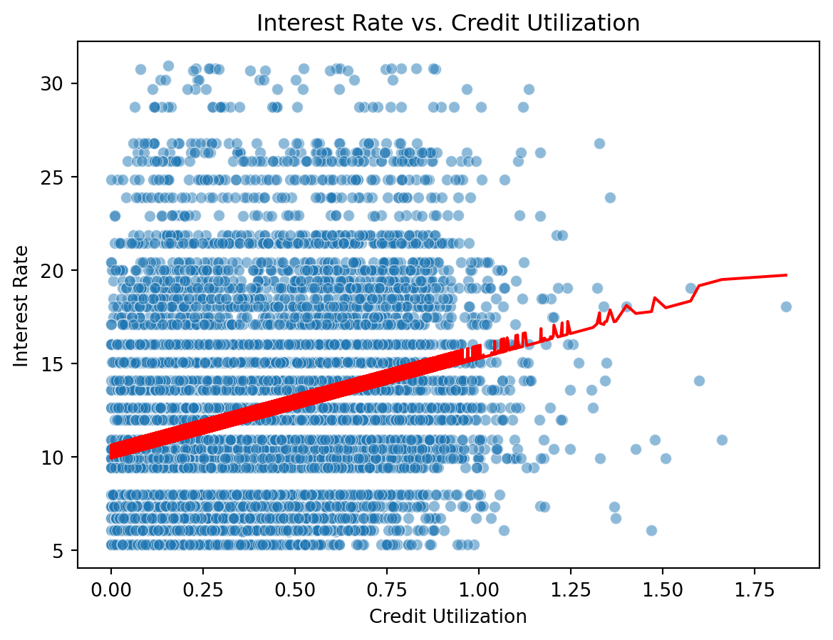

• Your turn: Interpret the intercept and the slope.

Answer Intercept: Renters with 0 credit utilization are predicted to have an interest rate of 9.93%.

Slope: For every 1.0 increase in credit utilization (which corresponds to a 100 percentage point increase — an unrealistic but technically accurate unit), the interest rate increases by 5.34 percentage points..

Interest rate vs. homeownership

Next we predict interest rates from homeownership, which is a categorical predictor with three levels:

homeownership_levels = loans['homeownership'].cat.categories
print(homeownership_levels)

Index(['Rent', 'Mortgage', 'Own'], dtype='object')

• Fit the linear regression model to predict interest rate from homeownership and display a summary of the model. Write the estimated model output below.

# Fit linear regression model
model_homeownership = smf.ols('interest_rate ~ C(homeownership)', data=loans).fit()


# Display summary
model_homeownership.summary()

OLS Regression Results

Dep. Variable:	interest_rate	R-squared:	0.006
Model:	OLS	Adj. R-squared:	0.006
Method:	Least Squares	F-statistic:	32.65
Date:	Mon, 05 May 2025	Prob (F-statistic):	7.35e-15
Time:	17:48:39	Log-Likelihood:	-30253.
No. Observations:	10000	AIC:	6.051e+04
Df Residuals:	9997	BIC:	6.053e+04
Df Model:	2
Covariance Type:	nonrobust

	coef	std err	t	P>|t|	[0.025	0.975]
Intercept	12.9250	0.080	161.033	0.000	12.768	13.082
C(homeownership)[T.Mortgage]	-0.8661	0.108	-8.030	0.000	-1.078	-0.655
C(homeownership)[T.Own]	-0.6110	0.158	-3.879	0.000	-0.920	-0.302

Omnibus:	1045.136	Durbin-Watson:	1.990
Prob(Omnibus):	0.000	Jarque-Bera (JB):	1408.154
Skew:	0.866	Prob(JB):	1.67e-306
Kurtosis:	3.615	Cond. No.	3.99

Notes:
[1] Standard Errors assume that the covariance matrix of the errors is correctly specified.

• Your turn: Interpret each coefficient in context of the problem.

Answer * All coefficients are statistically significant (p < 0.001), suggesting that homeownership status meaningfully affects predicted interest rates.

• Borrowers who don’t rent (i.e., have a mortgage or own) tend to get slightly lower interest rates, possibly due to being perceived as more financially stable or less risky.

• The overall R-squared is low (0.006), so homeownership alone doesn’t explain much of the variance in interest rates — but it still has a measurable effect.

Interest rate vs. credit utilization and homeownership

Main effects model

• Fit a model to predict interest rate from credit utilization and homeownership, without an interaction effect between the two predictors. Display the summary output and write out the estimated regression equation.

# Fit linear regression model: interest_rate ~ credit_util + homeownership (no interaction)
model_main_effects = smf.ols('interest_rate ~ credit_util + C(homeownership)', data=loans).fit()

# Display summary
model_main_effects.summary()

OLS Regression Results

Dep. Variable:	interest_rate	R-squared:	0.068
Model:	OLS	Adj. R-squared:	0.068
Method:	Least Squares	F-statistic:	243.7
Date:	Mon, 05 May 2025	Prob (F-statistic):	1.25e-152
Time:	17:48:39	Log-Likelihood:	-29926.
No. Observations:	9998	AIC:	5.986e+04
Df Residuals:	9994	BIC:	5.989e+04
Df Model:	3
Covariance Type:	nonrobust

	coef	std err	t	P>|t|	[0.025	0.975]
Intercept	9.9250	0.140	70.850	0.000	9.650	10.200
C(homeownership)[T.Mortgage]	0.6956	0.121	5.759	0.000	0.459	0.932
C(homeownership)[T.Own]	0.1283	0.155	0.827	0.408	-0.176	0.433
credit_util	5.3356	0.207	25.727	0.000	4.929	5.742

Omnibus:	1150.070	Durbin-Watson:	1.981
Prob(Omnibus):	0.000	Jarque-Bera (JB):	1616.376
Skew:	0.900	Prob(JB):	0.00
Kurtosis:	3.800	Cond. No.	6.48

Notes:
[1] Standard Errors assume that the covariance matrix of the errors is correctly specified.

$\text{text{interest\_rate}=9.93 + 5.34 cdot text{credit\_util} + 0.70 cdot text{Mortgage} + 0.13 cdot text{own}}$

• Write the estimated regression equation for loan applications from each of the homeownership groups separately.
  • Rent: $\text{text{interest\_rate} = 9.925 + 5.336 cdot text{credit\_util}}$
  • Mortgage: $\text{text{interest\_rate} = (9.925 + 0.696) + 5.336 cdot text{credit\_util} = 10.621 + 5.336 cdot text{credit\_util}}$
  • Own: $\text{text{interest\_rate} = (9.925 + 0.128) + 5.336 cdot text{credit\_util} = 10.053 + 5.336 cdot text{credit\_util}}$

Answer:

• The slope for credit_util is the same across all groups: 5.336.
  This means that as credit utilization increases, interest rates increase at the same rate, regardless of homeownership status.

• The difference lies in the intercepts:

  • Renters start at 9.93%
  • Mortgage holders start higher, at 10.62%
  • Homeowners who own outright start at 10.05%, but this difference is not statistically significant (p = 0.41)

Conclusion:
While credit utilization has a consistent impact on interest rate across all groups, the baseline rate varies slightly by homeownership — with mortgage holders paying the most on average. However, the effect of owning outright is minimal and not significant in this model.

Interaction effects model

• Fit a model to predict interest rate from credit utilization and homeownership, with an interaction effect between the two predictors. Display the summary output and write out the estimated regression equation.

# Fit linear regression model with interaction
model_interaction = smf.ols('interest_rate ~ credit_util * C(homeownership)', data=loans).fit()

# Display summary
model_interaction.summary()

OLS Regression Results

Dep. Variable:	interest_rate	R-squared:	0.069
Model:	OLS	Adj. R-squared:	0.069
Method:	Least Squares	F-statistic:	149.0
Date:	Mon, 05 May 2025	Prob (F-statistic):	4.79e-153
Time:	17:48:39	Log-Likelihood:	-29919.
No. Observations:	9998	AIC:	5.985e+04
Df Residuals:	9992	BIC:	5.989e+04
Df Model:	5
Covariance Type:	nonrobust

	coef	std err	t	P>|t|	[0.025	0.975]
Intercept	9.4369	0.199	47.526	0.000	9.048	9.826
C(homeownership)[T.Mortgage]	1.3903	0.228	6.109	0.000	0.944	1.836
C(homeownership)[T.Own]	0.6972	0.316	2.204	0.028	0.077	1.317
credit_util	6.2043	0.325	19.077	0.000	5.567	6.842
credit_util:C(homeownership)[T.Mortgage]	-1.6354	0.457	-3.577	0.000	-2.532	-0.739
credit_util:C(homeownership)[T.Own]	-1.0594	0.590	-1.797	0.072	-2.215	0.096

Omnibus:	1157.460	Durbin-Watson:	1.984
Prob(Omnibus):	0.000	Jarque-Bera (JB):	1630.777
Skew:	0.903	Prob(JB):	0.00
Kurtosis:	3.808	Cond. No.	19.2

Notes:
[1] Standard Errors assume that the covariance matrix of the errors is correctly specified.

$$\text{text{interest\_rate} = 9.437 + 6.204 cdot text{credit\_util} + 1.390 cdot text{Mortgage} + 0.697 cdot text{Own} - 1.635 cdot (text{credit\_util} times text{Mortgage}) - 1.059 cdot (text{credit\_util} times text{Own})}$$

$\text{text{interest\_rate} = 9.437 + 6.204 cdot text{credit\_util} + 1.390 cdot text{Mortgage} + 0.697 cdot text{Own} - 1.635 cdot (text{credit\_util} times text{Mortgage}) - 1.059 cdot (text{credit\_util} times text{Own})}$

• Write the estimated regression equation for loan applications from each of the homeownership groups separately.
  • Rent: $\text{text{interest\_rate} = 9.437 + 6.204 cdot text{credit\_util}}$
  • Mortgage: $\text{text{interest\_rate} = (9.437 + 1.390) + (6.204 - 1.635) cdot text{credit\_util} = 10.827 + 4.569 cdot text{credit\_util}}$
  • Own: $\text{text{interest\_rate} = (9.437 + 0.697) + (6.204 - 1.059) cdot text{credit\_util} = 10.134 + 5.145 cdot text{credit\_util}}$
• Question: How does the model predict the interest rate to vary as credit utilization varies for loan applicants with different homeownership status. Are the rates the same or different?

Answer:

No, the rates are not the same — the effect of credit utilization on interest rate varies depending on homeownership status, due to the interaction terms:

• Renters: Each 1-unit increase in credit utilization increases the interest rate by 6.20 percentage points.
• Mortgage holders: The slope is reduced to 4.57, meaning their interest rates increase more slowly with higher credit utilization.
• Owners: The slope is 5.15, slightly lower than renters but higher than mortgage holders.

Conclusion:
Renters are penalized most steeply for higher credit utilization, while those with a mortgage experience a more modest rate increase. This suggests that homeownership moderates the impact of credit utilization, likely because lenders view homeowners as lower-risk borrowers.

Choosing a model

Rule of thumb: Occam’s Razor - Don’t overcomplicate the situation! We prefer the simplest best model.

# Compare the main effects model and the interaction model
print("Main effects model AIC:", model_main_effects.aic)
print("Interaction effects model AIC:", model_interaction.aic)
print("Main effects model Adj. R²:", model_main_effects.rsquared_adj)
print("Interaction model Adj. R²:", model_interaction.rsquared_adj)

Main effects model AIC: 59859.377892328295
Interaction effects model AIC: 59850.400228039085
Main effects model Adj. R²: 0.0678893487525869
Interaction model Adj. R²: 0.06891213837091581

• Review: What is R-squared? What is adjusted R-squared?

R-squared $(R^2)$ is the proportion of the variance in the dependent variable (here, interest rate) that is explained by the independent variables in the model. It ranges from 0 to 1, with higher values indicating a better model fit.

Adjusted R-squared accounts for the number of predictors in the model. It adjusts $(R^2)$ downward if unnecessary variables are added. This helps prevent overfitting and is more appropriate for comparing models with different numbers of predictors.

• Question: Based on the adjusted $R^2$s of these two models, which one do we prefer?

Answer:

- Main effects model Adj. $(R^2)$: 0.0679
- Interaction model Adj. $(R^2)$: 0.0689

The interaction model has a slightly higher adjusted $(R^2)$, indicating it explains more variance in interest rates after accounting for model complexity. However, the improvement is very small (0.0689 vs. 0.0679), and the AIC difference is only ~9 points.

Thus, while the interaction model performs slightly better, according to Occam’s Razor, we may still prefer the main effects model unless the interaction effect is of specific interest or improves interpretability.

Another model to consider

• Your turn: Let’s add one more model to the variable – issue month. Should we add this variable to the interaction effects model from earlier?

model_with_month = smf.ols('interest_rate ~ credit_util * C(homeownership) + C(issue_month)', data=loans).fit()
print(model_with_month.summary())

                            OLS Regression Results                            
==============================================================================
Dep. Variable:          interest_rate   R-squared:                       0.069
Model:                            OLS   Adj. R-squared:                  0.069
Method:                 Least Squares   F-statistic:                     106.5
Date:                Mon, 05 May 2025   Prob (F-statistic):          5.62e-151
Time:                        17:48:39   Log-Likelihood:                -29919.
No. Observations:                9998   AIC:                         5.985e+04
Df Residuals:                    9990   BIC:                         5.991e+04
Df Model:                           7                                         
Covariance Type:            nonrobust                                         
============================================================================================================
                                               coef    std err          t      P>|t|      [0.025      0.975]
------------------------------------------------------------------------------------------------------------
Intercept                                    9.4870      0.211     44.861      0.000       9.072       9.902
C(homeownership)[T.Mortgage]                 1.3921      0.228      6.115      0.000       0.946       1.838
C(homeownership)[T.Own]                      0.7000      0.316      2.212      0.027       0.080       1.320
C(issue_month)[T.Jan-2018]                  -0.0799      0.121     -0.660      0.509      -0.317       0.157
C(issue_month)[T.Mar-2018]                  -0.0651      0.119     -0.546      0.585      -0.299       0.169
credit_util                                  6.2043      0.325     19.075      0.000       5.567       6.842
credit_util:C(homeownership)[T.Mortgage]    -1.6384      0.457     -3.583      0.000      -2.535      -0.742
credit_util:C(homeownership)[T.Own]         -1.0646      0.590     -1.805      0.071      -2.221       0.091
==============================================================================
Omnibus:                     1157.710   Durbin-Watson:                   1.984
Prob(Omnibus):                  0.000   Jarque-Bera (JB):             1631.442
Skew:                           0.903   Prob(JB):                         0.00
Kurtosis:                       3.809   Cond. No.                         20.8
==============================================================================

Notes:
[1] Standard Errors assume that the covariance matrix of the errors is correctly specified.

Answer Based on the output of model_with_month, here’s how to interpret whether or not to keep issue_month in the model:

Adjusted R²: - Interaction model (no month): 0.0689
- With issue_month added: 0.0690
➡️ Change: +0.0001 — a negligible increase in adjusted R².

AIC Comparison: - Interaction model AIC: 59850.40
- Model with issue_month AIC: 59850.00
➡️ AIC improved by only 0.4 points, which is not meaningful.

Coefficient Significance for issue_month: - Only 2 months are shown (Jan-2018, Mar-2018), and both have high p-values (> 0.5), meaning they are not statistically significant predictors.

Conclusion (based on Occam’s Razor):

Although adding issue_month results in a tiny improvement in AIC and adjusted R², the predictive value is negligible and the coefficients for months shown are not significant.

Therefore, we should not include issue_month in the final model.
The interaction model without it is simpler and performs just as well — and thus is the preferred model.