import pandas as pd
import matplotlib.pyplot as plt
import seaborn as sns

infosci = pd.read_csv("data/degrees.csv")AE 05: Wrangling College Majors
Suggested answers
Application exercise
Answers
Important
These are suggested answers. This document should be used as reference only, it’s not designed to be an exhaustive key.
Goal
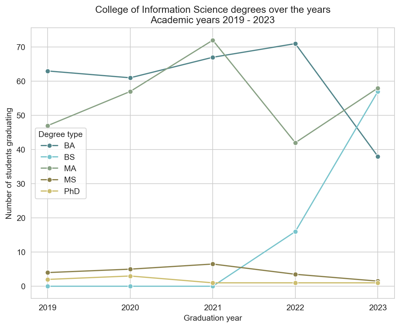
Our ultimate goal in this application exercise is to make the following data visualization.
Data
For this exercise you will work with data on the proportions of Bachelor’s degrees awarded in the US between 2005 and 2015. The dataset you will use is in your data/ folder and it’s called degrees.csv.
And let’s take a look at the data.
infosci.head()| degree | 2019 | 2020 | 2021 | 2022 | 2023 | |
|---|---|---|---|---|---|---|
| 0 | Information Science & eSociety (BA) | 63.0 | 61.0 | 67.0 | 71 | 38 |
| 1 | Information Science (BS) | NaN | NaN | NaN | 16 | 57 |
| 2 | Information (PhD) | 2.0 | 3.0 | 1.0 | 1 | 1 |
| 3 | Library & Information Science (MA) | 47.0 | 57.0 | 72.0 | 42 | 58 |
| 4 | Information (MS) | 8.0 | 10.0 | 13.0 | 5 | 2 |
Pivoting
- Pivot the
degreesdata frame longer such that each row represents a degree type / year combination andyearandnumber of graduates for that year are columns in the data frame.
infosci_long = infosci.melt(id_vars='degree', var_name='year', value_name='n')

infosci_long.info()
<class 'pandas.core.frame.DataFrame'>
RangeIndex: 30 entries, 0 to 29
Data columns (total 3 columns):
# Column Non-Null Count Dtype
--- ------ -------------- -----
0 degree 30 non-null object
1 year 30 non-null object
2 n 24 non-null float64
dtypes: float64(1), object(2)
memory usage: 848.0+ bytes- Question: What is the type of the
yearvariable? Why? What should it be?
It’s an object variable since the information came from the columns of the original data frame and Python cannot know that these character strings represent years. The variable type should be numeric (int64).
- Start over with pivoting, and this time also make sure
yearis a numerical variable in the resulting data frame.
infosci_long = infosci.melt(id_vars='degree', var_name='year', value_name='n')
infosci_long['year'] = pd.to_numeric(infosci_long['year'])

infosci_long.info()
<class 'pandas.core.frame.DataFrame'>
RangeIndex: 30 entries, 0 to 29
Data columns (total 3 columns):
# Column Non-Null Count Dtype
--- ------ -------------- -----
0 degree 30 non-null object
1 year 30 non-null int64
2 n 24 non-null float64
dtypes: float64(1), int64(1), object(1)
memory usage: 848.0+ bytes- Question: What does an
NaNmean in this context? Hint: The data come from the university registrar, and they have records on every single graduates, there shouldn’t be anything “unknown” to them about who graduated when.
NAs should actually be 0s.
- Add on to your pipeline that you started with pivoting and convert
NaNs innto0s.
infosci_long = infosci.melt(id_vars='degree', var_name='year', value_name='n')
infosci_long['year'] = pd.to_numeric(infosci_long['year'])
infosci_long['n'] = infosci_long['n'].fillna(0)

infosci_long.isna().sum()
degree 0
year 0
n 0
dtype: int64- In our plot the degree types are BA, BS, MA, MS, and PhD. This information is in our dataset, in the
degreecolumn, but this column also has additional characters we don’t need. Create a new column calleddegree_typewith levels BA, BS, MA, MS, and PhD (in this order) based ondegree. Do this by adding on to your pipeline from earlier.
infosci_long = infosci.melt(id_vars='degree', var_name='year', value_name='n')
infosci_long['year'] = pd.to_numeric(infosci_long['year'])
infosci_long['n'] = infosci_long['n'].fillna(0)

infosci_long[['major', 'degree_type']] = infosci_long['degree'].str.split(' \(', expand=True)
infosci_long['degree_type'] = infosci_long['degree_type'].str.replace('\)', '', regex=True)

degree_order = pd.CategoricalDtype(categories=["BA", "BS", "MA", "MS", "PhD"], ordered=True)
infosci_long['degree_type'] = infosci_long['degree_type'].astype(degree_order)

infosci_long.head()| degree | year | n | major | degree_type | |
|---|---|---|---|---|---|
| 0 | Information Science & eSociety (BA) | 2019 | 63.0 | Information Science & eSociety | BA |
| 1 | Information Science (BS) | 2019 | 0.0 | Information Science | BS |
| 2 | Information (PhD) | 2019 | 2.0 | Information | PhD |
| 3 | Library & Information Science (MA) | 2019 | 47.0 | Library & Information Science | MA |
| 4 | Information (MS) | 2019 | 8.0 | Information | MS |
- Now we start making our plot, but let’s not get too fancy right away. Create the following plot, which will serve as the “first draft” on the way to our Goal. Do this by adding on to your pipeline from earlier.
sns.set_style("darkgrid")

plt.figure(figsize=(8, 6))
sns.lineplot(data=infosci_long, x='year', y='n', hue='degree_type', ci=None, marker='o')
plt.legend()
plt.show()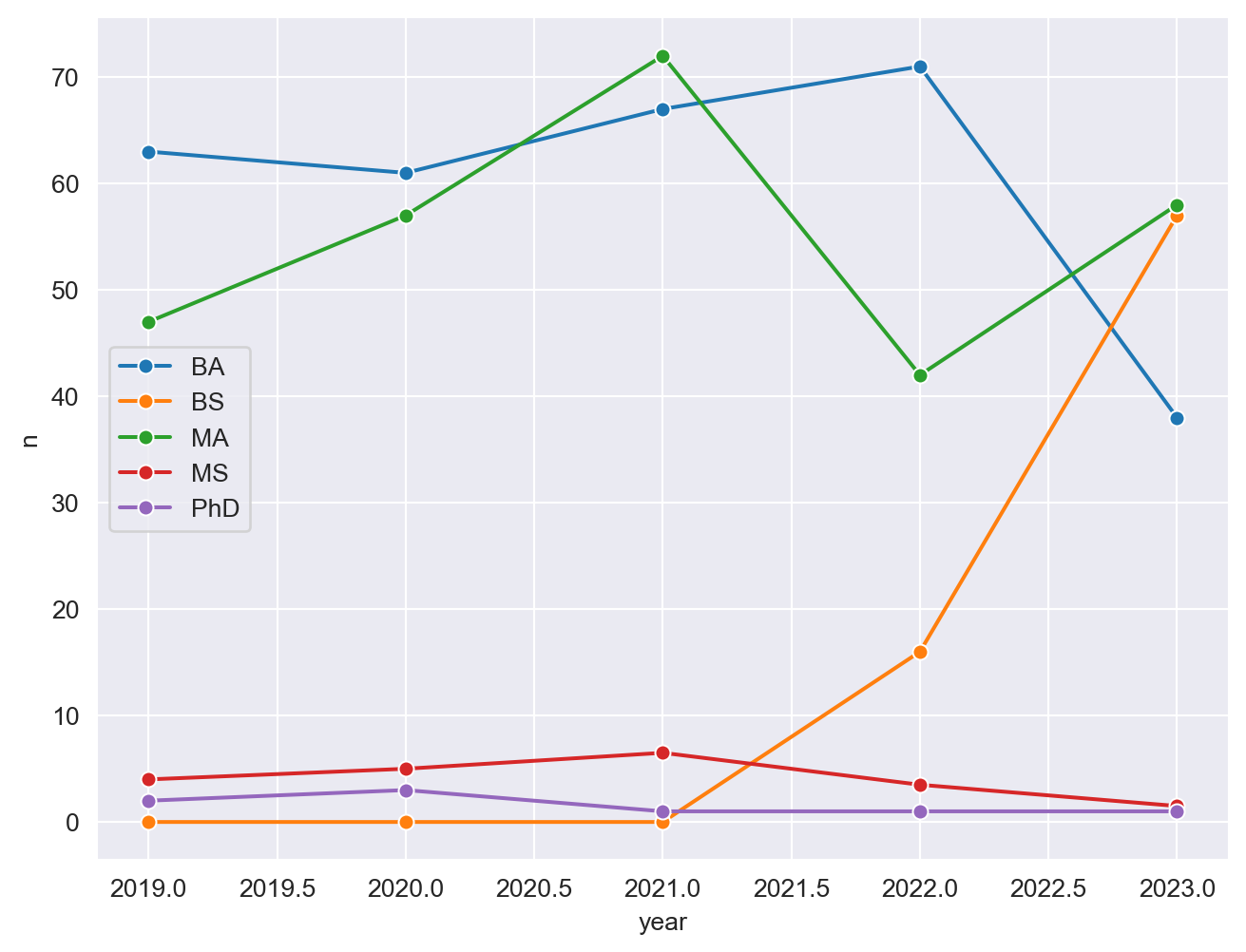
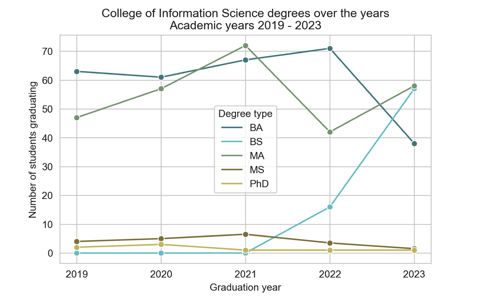
What aspects of the plot need to be updated to go from the draft you created above to the Goal plot at the beginning of this application exercise.
x-axis scale: need to go from 2019 to 2023 in unique year values
line colors
axis labels: title, x, y
theme
Update x-axis scale such that the years displayed go from 2019 to 2023 in unique years. Do this by adding on to your pipeline from earlier.
plt.figure(figsize=(8, 6))
sns.lineplot(data=infosci_long, x='year', y='n', hue='degree_type', ci=None, marker='o')
plt.xticks(ticks=infosci_long['year'].unique(), labels=infosci_long['year'].unique())
plt.legend()
plt.show()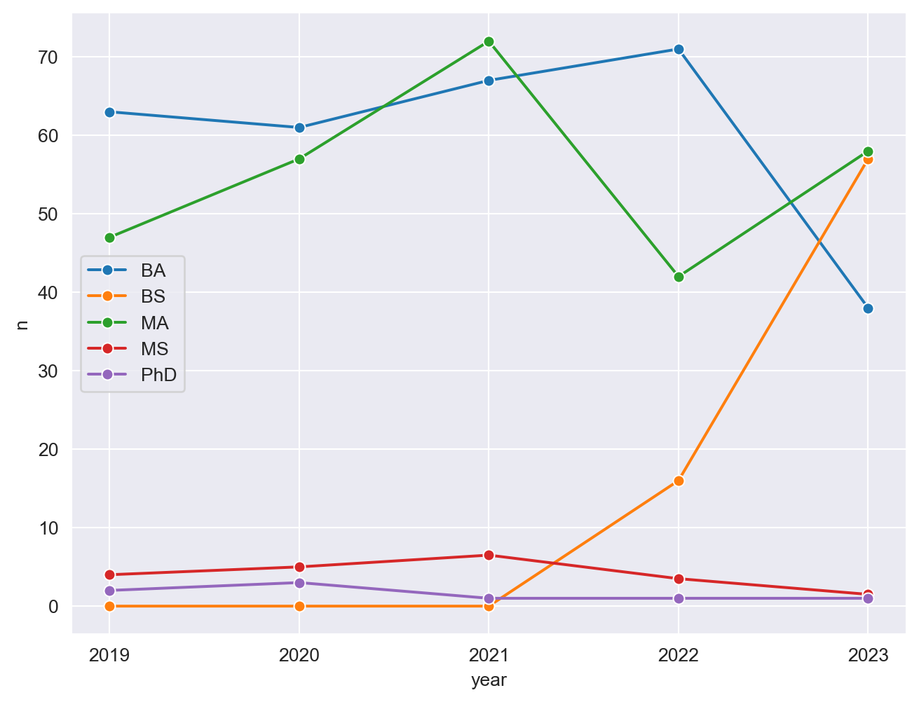
Update line colors using the following level / color assignments. Once again, do this by adding on to your pipeline from earlier.
BA: “#53868B”
BS: “#7AC5CD”
MA: “#89a285”
MS: “#8B814C”
PhD: “#CDBE70”
custom_palette = {
    "BA": "#53868B",
    "BS": "#7AC5CD",
    "MA": "#89a285",
    "MS": "#8B814C",
    "PhD": "#CDBE70"
}

plt.figure(figsize=(8, 6))
sns.lineplot(data=infosci_long, x='year', y='n', hue='degree_type', ci=None, marker='o')
plt.xticks(ticks=infosci_long['year'].unique(), labels=infosci_long['year'].unique())
plt.legend()
plt.show()
- Update the plot labels (
title,x, andy) and usesns.set_style("white_grid"). Once again, do this by adding on to your pipeline from earlier.
sns.set_style("whitegrid")

custom_palette = {
    "BA": "#53868B",
    "BS": "#7AC5CD",
    "MA": "#89a285",
    "MS": "#8B814C",
    "PhD": "#CDBE70"
}

plt.figure(figsize=(8, 6))
sns.lineplot(data=infosci_long, x='year', y='n', hue='degree_type', ci=None, marker='o', palette=custom_palette)
plt.title('College of Information Science degrees over the years\nAcademic years 2019 - 2023')
plt.xticks(ticks=infosci_long['year'].unique(), labels=infosci_long['year'].unique())
plt.xlabel('Graduation year')
plt.ylabel('Number of students graduating')
plt.legend(title='Degree type')
plt.grid(True)
plt.show()