[3 2]Linear algebra I
Lecture 22
University of Arizona
INFO 511 - Spring 2025
Linear algebra
Linear algebra
Linear algebra is the study of vectors, vector spaces, and linear transformations.
Fundamental to many fields including data science, machine learning, and statistics.
Vectors
Vectors
Definition:
- Vectors are objects that can be added together and multiplied by scalars to form new vectors. In a data science context, vectors are often used to represent numeric data.
Examples:
Three-dimensional vector: [height, weight, age] = [70, 170, 40]
Four-dimensional vector: [exam1, exam2, exam3, exam4] = [95, 80, 75, 62]
Vectors in Python
Vector addition
Vectors of the same length can be added or subtracted componentwise.
Example: \(\mathbf{v} = [3,2]\) and \(\mathbf{w}=[2,-1]\)
Result: \(\mathbf{v}+\mathbf{w}=[5,1]\)
Code
v = np.array([3, 2])
w = np.array([2, -1])
v_plus_w = v + w

plt.quiver(*origin, *v, color='r', scale=1, scale_units='xy', angles='xy')
plt.quiver(*origin, *w, color='b', scale=1, scale_units='xy', angles='xy')
plt.quiver(*origin, *v_plus_w, color='g', scale=1, scale_units='xy', angles='xy')
plt.xlim(0, 6)
plt.ylim(-2, 3)
plt.grid()
plt.show()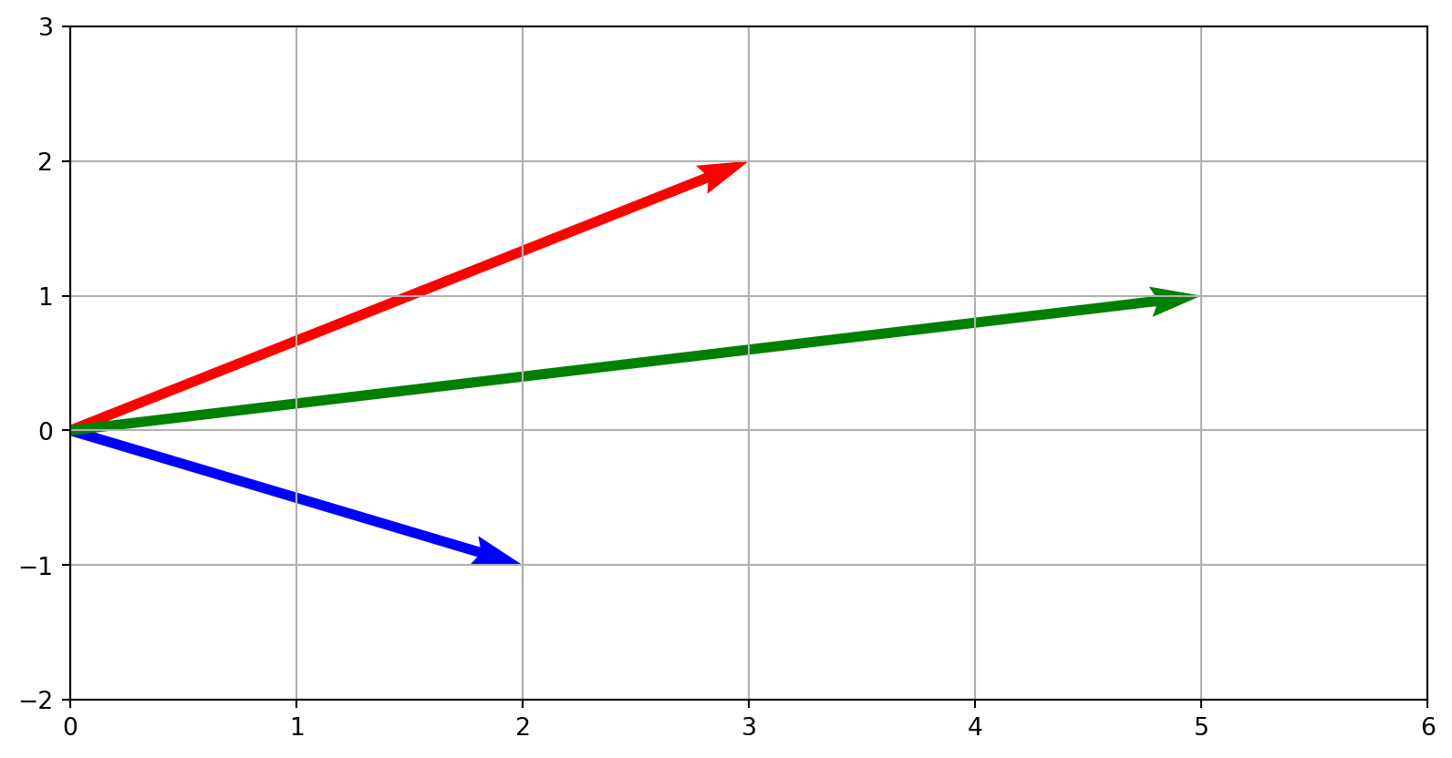
Vector subtraction
Vectors of the same length can be added or subtracted componentwise.
Example: \(\mathbf{v} = [3,2]\) and \(\mathbf{w}=[2,-1]\)
Result: \(\mathbf{v}-\mathbf{w}=[1,3]\)
Code
v = np.array([3, 2])
w = np.array([2, -1])
v_plus_w = v - w

plt.quiver(*origin, *v, color='r', scale=1, scale_units='xy', angles='xy')
plt.quiver(*origin, *w, color='b', scale=1, scale_units='xy', angles='xy')
plt.quiver(*origin, *v_plus_w, color='g', scale=1, scale_units='xy', angles='xy')
plt.xlim(0, 6)
plt.ylim(-2, 3)
plt.grid()
plt.show()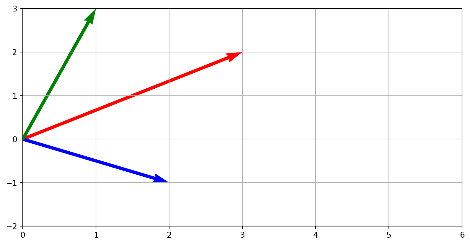
Vector scaling
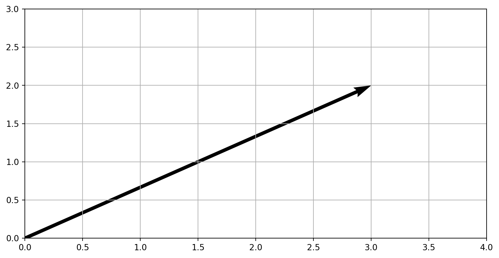
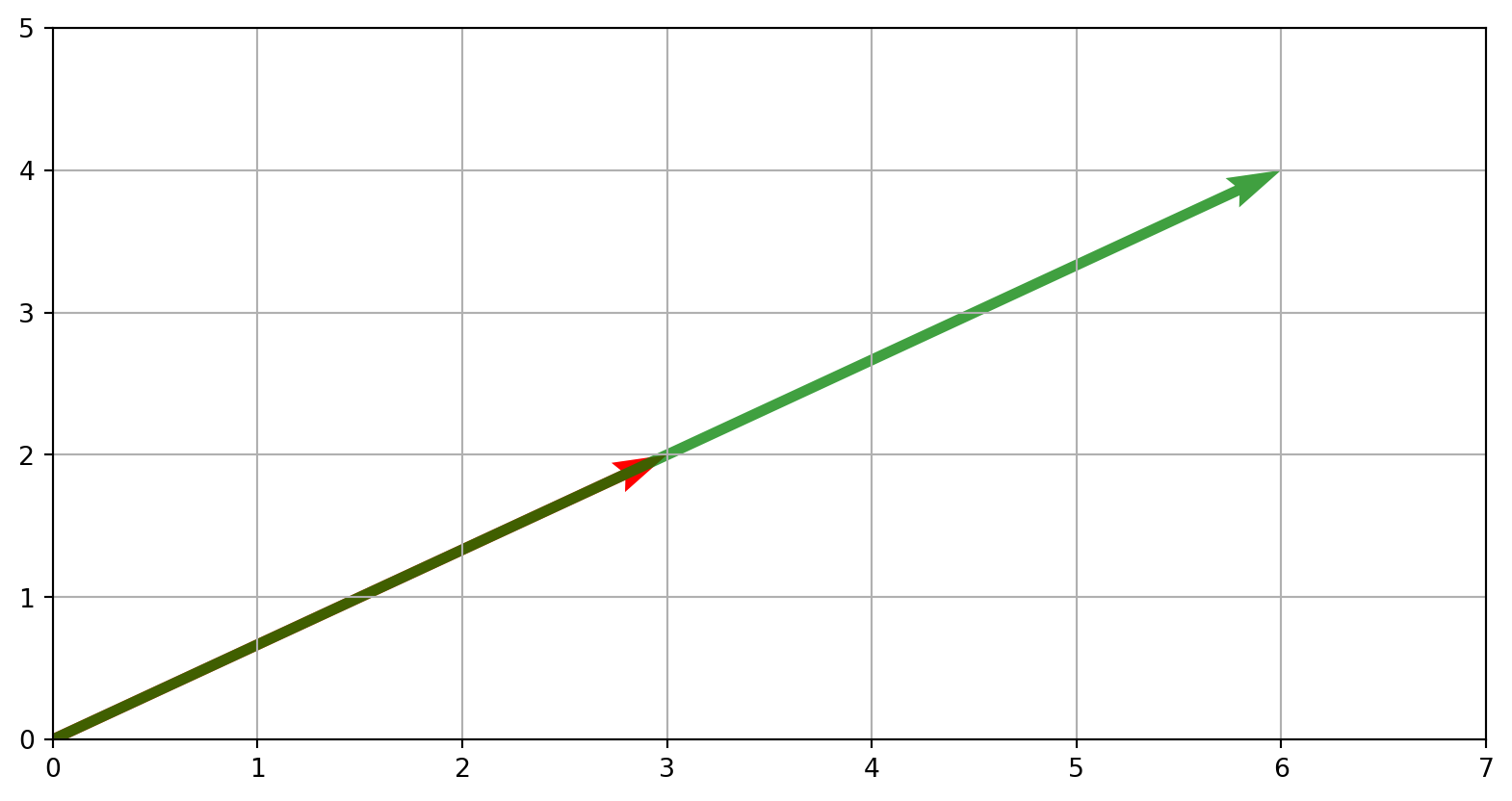
Scaling vector \(\mathbf{v}=[3,2]\) by \(2\)
Result: \([6,4]\)
Linearly independent and span
Span
The span of a set of vectors \(\mathbf{v1},\mathbf{v2},...,\mathbf{vn}\) is the set of all linear combinations of the vectors.
i.e., all the vectors \(\mathbf{b}\) for which the equation \([\mathbf{v1} \space \mathbf{v2} \space... \space\mathbf{vn}]\mathbf{x=b}\)
Linear independent vs. dependent
Vectors are linearly independent if each vector lies outside the span of the remaining vectors. Otherwise, the vectors are said to be linearly dependent1.
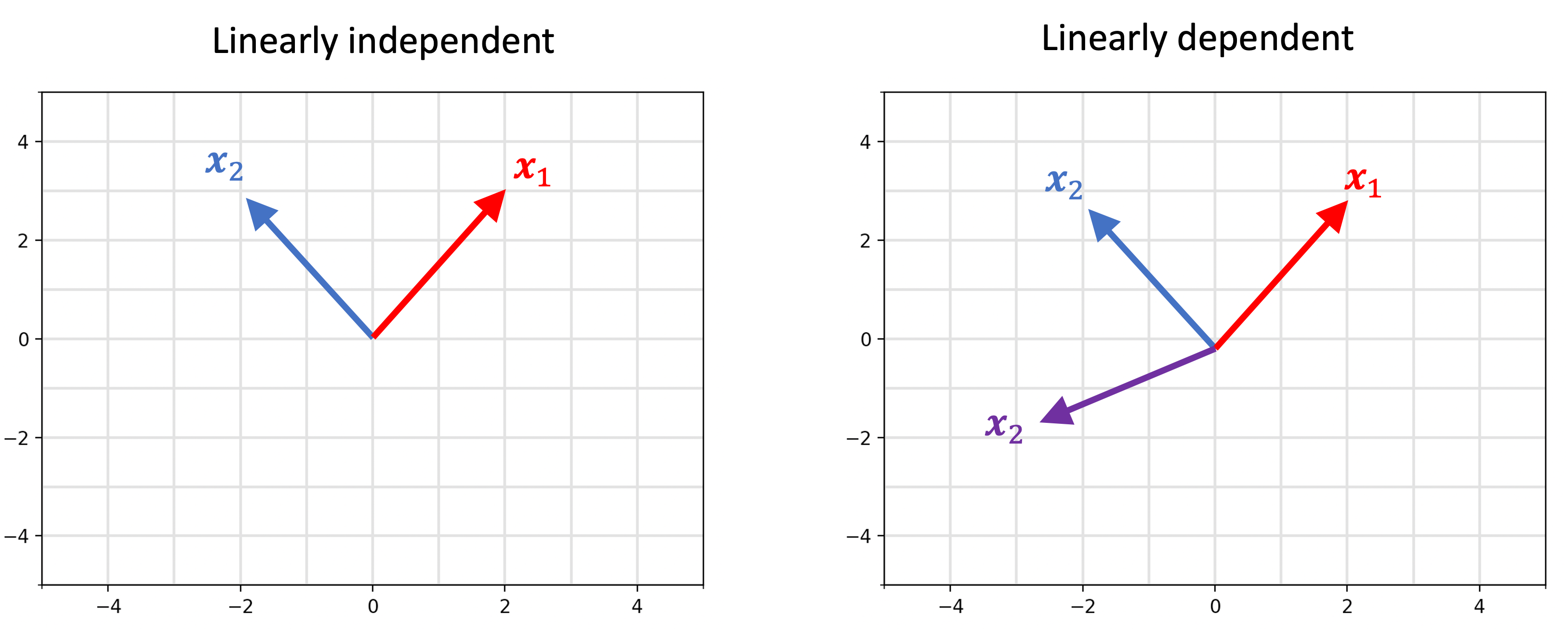
Linear independent vs. dependent
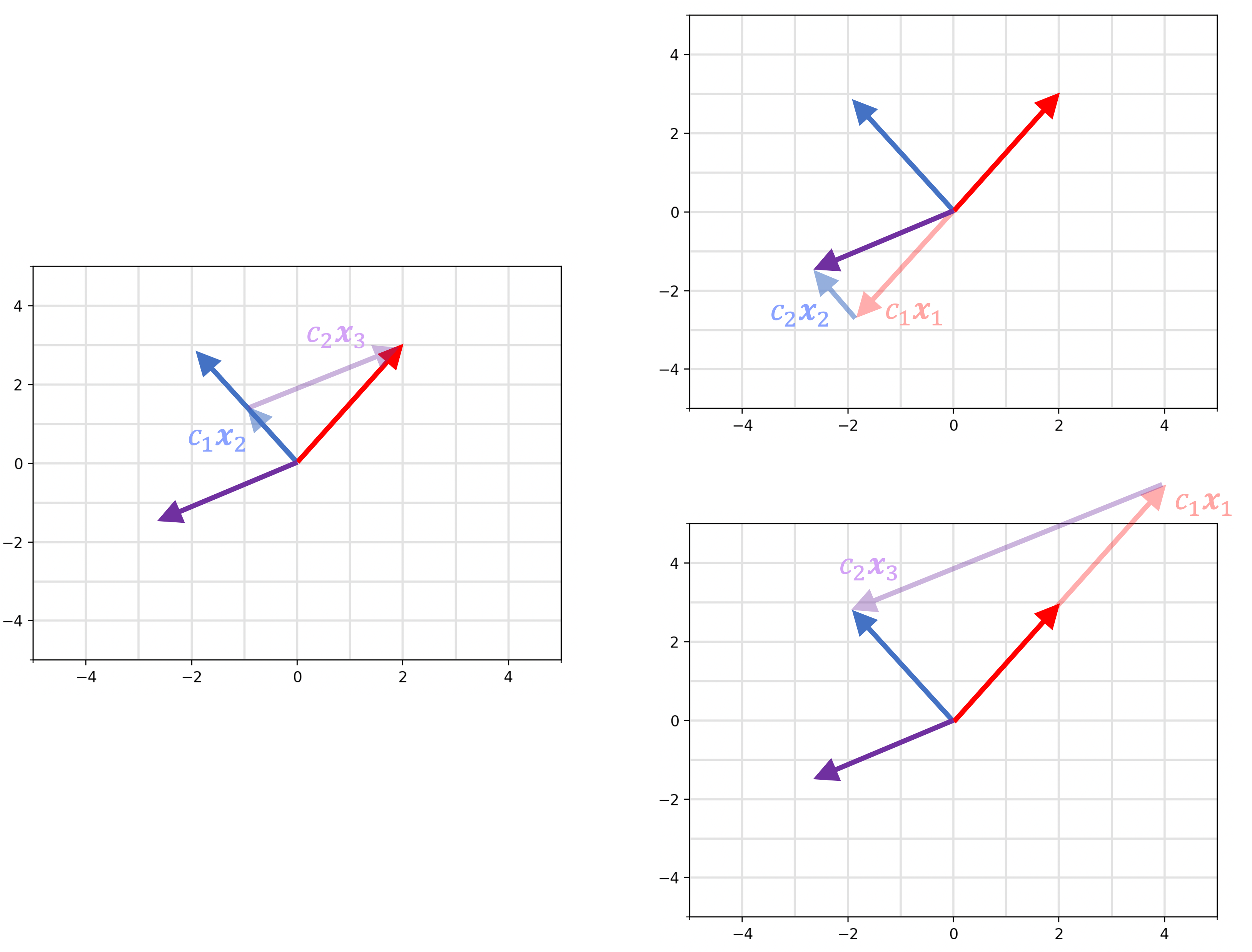
The vector on th right can be constructed by any two combination of the other vectors.
Matrices
Matrices
Matrix transposition
Matrix transposition involves swapping the rows and columns.
Notation: If \(\mathbf{A}\) is a matrix, then its transpose is denoted as \(\mathbf{A}^T\).
Given the matrix \(\mathbf{A}\):
\[ \mathbf{A}= \begin{bmatrix}a_{11} & a_{12} & a_{13}\\a_{21} & a_{22} & a_{23}\\a_{31} & a_{32} & a_{33}\end{bmatrix} \]
- The matrix \(\mathbf{A}^T\) is:
\[ \mathbf{A}^T=\begin{bmatrix}a_{11} & a_{21} & a_{31}\\a_{12} & a_{22} & a_{32}\\a_{13} & a_{23} & a_{33}\end{bmatrix} \]
Matrix transposition: Python
Matrix-vector multiplication
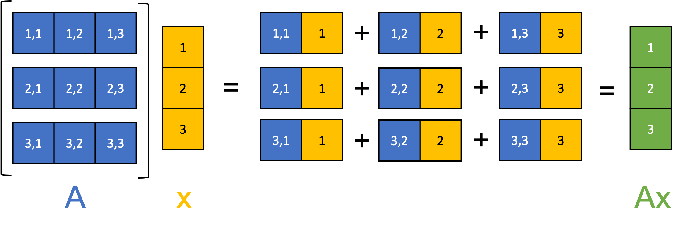
Matrix-vector multiplication
Geometrically
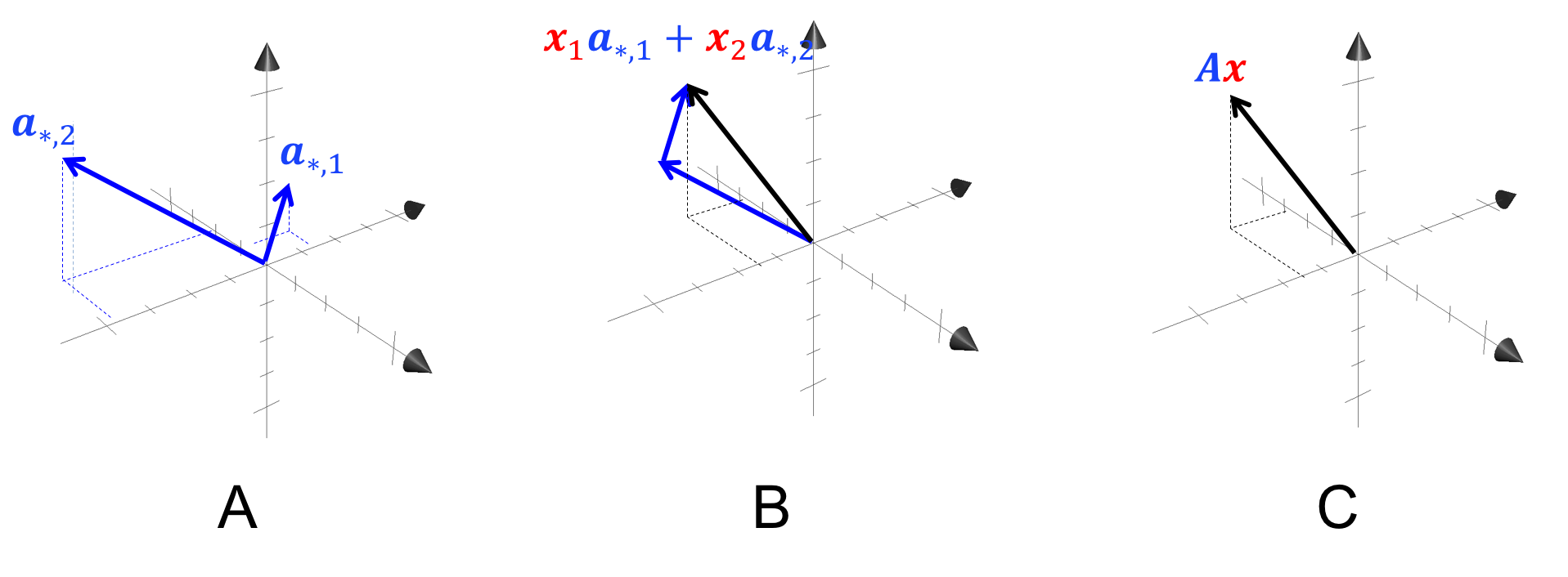
Matrix-vector multiplication
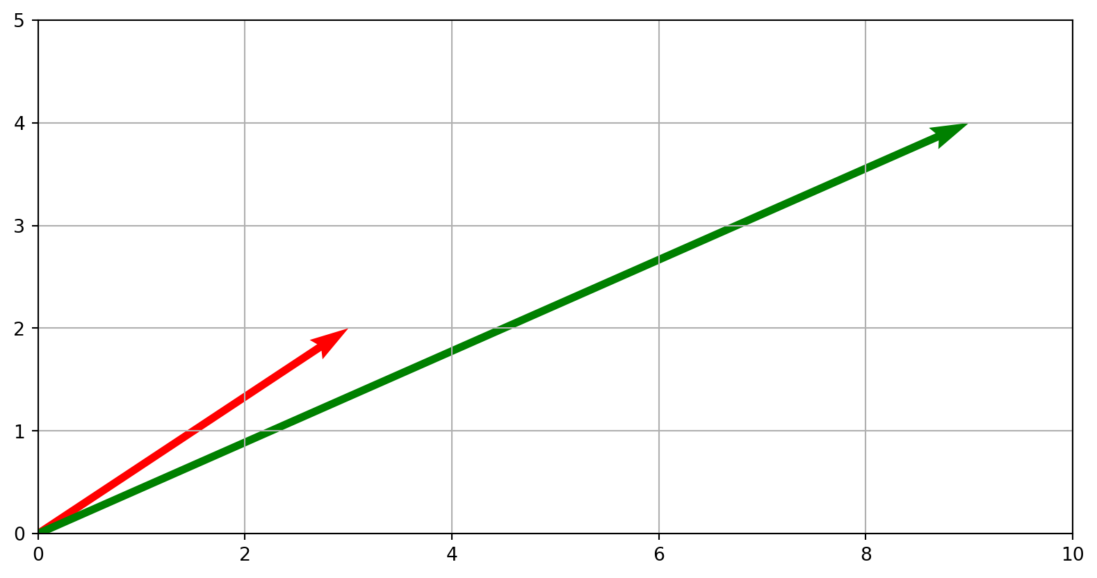
Matrix-vector multiplication transforms the vector according to the basis vectors of the matrix.
Formula: \(\mathbf{A} \cdot \mathbf{v}\)
\[ \mathbf{A} \cdot \mathbf{v} = \begin{bmatrix}3 & 0 \\0 & 2 \end{bmatrix} \cdot [3, 2] \]
Determinants
The determinant is a function that maps square matrices to real numbers: \(\text{Det}:ℝ^{m×m}→ℝ\)
where the absolute value of the determinant describes the volume of the parallelepided formed by the matrix’s columns.
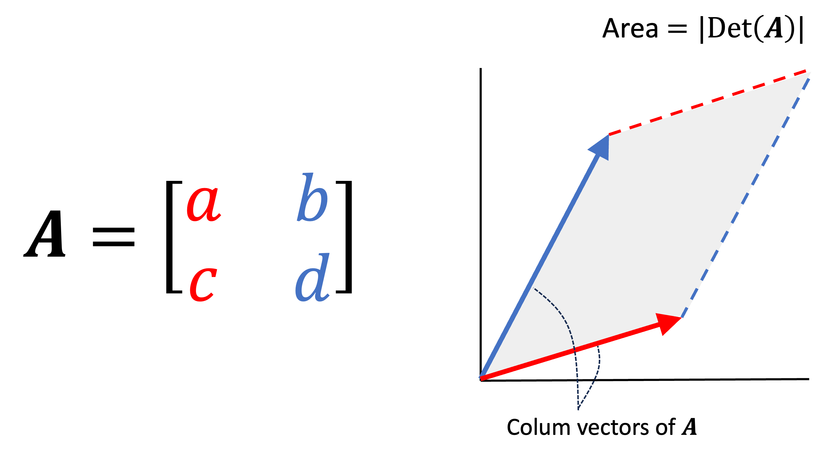
Determinants: Python
Determinants measure the scale factor of a transformation.
Determinant of 0 indicates linear dependence.
ae-15-linear-algebra
Practice matrix operations (you will be tested on this in Exam 2)
